Jupyter Notebook - python based lab book
Data analysis using Jupyter Notebook. Natural sciences more and more rely on skills related to Data Science. Experiments produce more and more data, and skilled researcher has to know how to deal with variety of data and sometime very large datasets. Anaconda Python Distribution offers large set of great tools to manipulate any kind of data “out of the box”. Multitude of community packages allows to read, analyze and report all kinds of data produced by science. It is caused mostly by simple fact, that scientific community is developing it’s tools mostly in Python. How to work with small and large data in python and make Jupyter Notebook your lab-book? Check this article.
Install Anaconda
Data Science skills are essential for every decent researcher.
Anaconda Python Distribution prepared by Continuum Analytics is the most comprehensive and free bundle of Python software dedicated to Data Science.
I strongly recommended to use Anaconda distribution, which will install Python interpreter, the Jupyter Notebook, and several other packages commonly used in data science and this tutorial. If you choose Anaconda 3, your interpreter will be of version 3.6 (current version) or higher (3.7 alpha is already available).
Execute script and just follow instructions from installation program (your current version may differ from the one listed here):
> wget https://repo.continuum.io/archive/Anaconda3-4.3.1-Linux-x86_64.sh

--2017-03-03 19:36:37--  https://repo.continuum.io/archive/Anaconda3-4.3.1-Linux-x86_64.sh
Resolving repo.continuum.io (repo.continuum.io)... 104.16.18.10, 104.16.19.10, 2400:cb00:2048:1::6810:130a, ...
Connecting to repo.continuum.io (repo.continuum.io)|104.16.18.10|:443... connected.
HTTP request sent, awaiting response... 200 OK
Length: 497343851 (474M) [application/x-sh]
Saving to: 'Anaconda3-4.3.1-Linux-x86_64.sh'

Anaconda3-4.3.1-Linux-x86_64.sh     100%[==========================================>] 474.30M  14.1MB/s in 34s

2017-03-03 19:37:12 (13.8 MB/s) - 'Anaconda3-4.3.1-Linux-x86_64.sh' saved [497343851/497343851]

> bash ./Anaconda3-4.3.1-Linux-x86_64.sh
To make sure software is up to date, run:
> conda update --allAnaconda will install nearly 200 packages (182 to be exact), including most important for this tutorial: Jupyter Notebook, ipython, pandas, numpy, statsmodels
Anaconda channels
conda is built in Anaconda package manager, which uses default, maintained by Continuum Analytics python packages repository. Some packages are distributed in repositories owned by groups other than Anaconda team. Repositories are called channels. One can indicate channel simply by choosing -c or --channel flag during invoking conda install command. Some of the channels are supported by continuum Analytics, like conda-forge, omnia or r. They are full of excellent packages developed by Anaconda community. Every time I mention I want to use other channel than default, conda will check this repositories for available packages. It is possible to add this channels to the .condarc file (see: here). First config file must be created by running conda config command. If other version of this file is placed in Anaconda installation root directory it will override users home configuration. to notify package manager, that every time I want to install something this channels should be checked. Order of repositories is important. In case packages are deployed to both repositories listed in channels section, last repository super-seeds all above it. Example file looks like this:
channels:
    - omnia
    - conda-forge
    - r
    - defaults

show_channel_urls: True

proxy_servers:
    http: http://user:pass@corp.com:8080
    https: https://user:pass@corp.com:8080
Last group of inputs is very important for users behind corporate proxy, which will block conda package lookup, unless correct settings are provided. Additionally one can alway use official python package manager pip in parallel to conda. Conda is able to sense origin of the package and shows this during package listing. Pip checks PyPI (Python Packages Index) repository for python packages (which stores nearly 110 000 packages).
Another great part about Anaconda and Jupyter Notebook. It is cross-platform, which means, that Notebook files created on one system will open on other system with similar package configuration.
Jupyter Notebook / Jupyter Lab
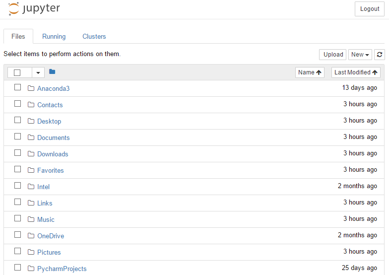
Jupyter Notebook allows to create and share documents that contain live code, equations, visualizations and explanatory text. Text may be written in markdown markup language. Code can produce rich output such as images, videos, LaTeX, and JavaScript. Interactive widgets can be used to manipulate and visualize data in real time.
Alternatively you may add path to the existing Jupyter notebook file with .ipybn extension. If you add path to the notebook file ( extension .ipynb), it will be opened in the location of the file. Jupyter automatically runs a local server.
> jupyter notebook

[I 21:09:38.658 NotebookApp] Serving notebooks from local directory: /home/mdyzma/
[I 21:09:38.659 NotebookApp] 0 active kernels
[I 21:09:38.660 NotebookApp] The Jupyter Notebook is running at: http://localhost:8888/?token=c6a93623006ede30a579af4d7e693909abd90c98224916ee
[I 21:09:38.660 NotebookApp] Use Control-C to stop this server and shut down all kernels (twice to skip confirmation). [C 21:09:38.665 NotebookApp]

    Copy/paste this URL into your browser when you connect for the first time,
    to login with a token:
        http://localhost:8888/?token=c6a93623006ede30a579af4d7e693909abd90c98224916ee
[I 21:09:39.005 NotebookApp] Accepting one-time-token-authenticated connection from ::1
It should start notebook server in your browser (default address: http://127.0.0.1:8888):
There is a handy collection of extensions that add functionality to the Jupyter notebook. Extensions are grouped in package nbextensions, which is not included in fresh Anaconda installation and I will install it using conda:
> conda install -c conda-forge jupyter_contrib_nbextensions
Fetching package metadata .............
Solving package specifications: .

Package plan for installation in environment /home/mdyzma/anaconda3:

The following NEW packages will be INSTALLED:

    jupyter_contrib_core:              0.3.1-py36_0   conda-forge
    jupyter_contrib_nbextensions:      0.2.8-py36_1   conda-forge
    jupyter_highlight_selected_word:   0.0.10-py36_0  conda-forge
    jupyter_latex_envs:                1.3.8.2-py36_1 conda-forge
    jupyter_nbextensions_configurator: 0.2.5-py36_0   conda-forge

The following packages will be UPDATED:

    conda:                             4.3.21-py36_0              --> 4.3.21-py36_1 conda-forge

The following packages will be SUPERSEDED by a higher-priority channel:

    conda-env:                         2.6.0-0                    --> 2.6.0-0       conda-forge

Proceed ([y]/n)? y


conda-env-2.6. 100% |###############################| Time: 0:00:00 206.58 kB/s
conda-4.3.21-p 100% |###############################| Time: 0:00:01 281.65 kB/s
jupyter_contri 100% |###############################| Time: 0:00:00 417.99 kB/s
jupyter_highli 100% |###############################| Time: 0:00:00 793.82 kB/s
jupyter_latex_ 100% |###############################| Time: 0:00:02 324.68 kB/s
jupyter_nbexte 100% |###############################| Time: 0:00:01 442.23 kB/s
jupyter_contri 100% |###############################| Time: 0:00:03   5.47 MB/s
Because I used conda it will automatically register all extensions and copy necessary javascript and css files in Jupyter environment for me. If I used pip instead, I would have to fetch additional command: jupyter contrib nbextension install --user
Jupyter Lab is new project of Jupyter team, which eventually will replace good old notebook, but currently it is in very early alpha release version and it is not recommended to be used in any serious project. It has built in file manager, image browser, documentation and many, many other. And one disadvantage: ipywidgets and nbextensions do not work yet or their functionality must be loaded through lab extensions system, which is not very convenient. Another handy extension is watermark package. It will timestamp notebooks and provide basic python configuration info. I will fetch latest version from GitHub:
> pip install -e git+https://github.com/rasbt/watermark#egg=watermark
Obtaining watermark from git+https://github.com/rasbt/watermark#egg=watermark
  Cloning https://github.com/rasbt/watermark to /home/mdyzma/watermark
Installing collected packages: watermark
  Running setup.py develop for watermark
Successfully installed watermark
Jupyter lab is not accessible in Anaconda distribution out of the box and must be installed. One can do it with default package manager from conda-forge channel:
> conda install -c conda-forge jupyterlab
Fetching package metadata .............
Solving package specifications: .

Package plan for installation in environment /home/mdyzma/anaconda3:

The following NEW packages will be INSTALLED:

    jupyterlab:          0.23.2-py36_0 conda-forge
    jupyterlab_launcher: 0.2.9-py36_0  conda-forge

The following packages will be SUPERSEDED by a higher-priority channel:

    conda:               4.3.21-py36_0             --> 4.3.21-py36_0 conda-forge
    conda-env:           2.6.0-0                   --> 2.6.0-0       conda-forge

Proceed ([y]/n)? y

conda-env-2.6. 100% |###############################| Time: 0:00:00  73.67 kB/s
conda-4.3.21-p 100% |###############################| Time: 0:00:01 378.40 kB/s
jupyterlab_lau 100% |###############################| Time: 0:00:00   1.18 MB/s
jupyterlab-0.2 100% |###############################| Time: 0:00:01   1.34 MB/s
Lab environment can be started using jupyter lab command. It should start in default browser under this address: http://127.0.0.1:8888.
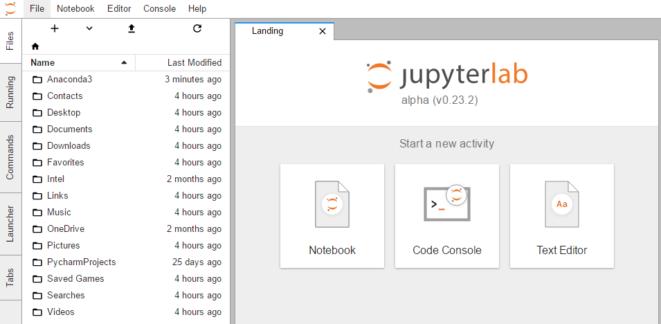
More information about this project and development plans can be found here.
Simple conda list shows all packages installed in current environment. Main tools I will use in this tutorial include:
numpy- array calculationssympy- symbolic mathematicsmatplotlib- 2D plottingstatsmodels- statistical modelspandas- data structures and analysis
which are part of SciPy - python based scientific ecosystem. Numpy and Pandas alone have enormous documentations, which are worth to check. Huge advantage of notebook environment is that it allows to compute and manipulate data directly and export entire notebook in various formats, to share with other. There is also JupyterHub, providing access to the notebook for multiple users, which can be used as a official project documentation in secure location and controlled access. Check JupyterHub documentation to learn more.
Experiments examples:
To present power enclosed in python and jupyter notebook I will create several scenarios of typical experiments conducted in labs. It will cover data acquisition, modeling, visualization and data storage.
Protein concentration
Example of simple experiment with data from VIS spectrophotometric experiment. Lets assume we have solution with protein colored by protein dye. For a uniform absorbing solution the proportion of light passing through is called the transmittance: \(T\), and the proportion of light absorbed by molecules in the medium is absorbance, \(Abs\). Experiment consists of three steps:
- Determine the absorption spectra \(\lambda_{max}\)
- Calculate the extinction coefficient (\(\epsilon\)) of the standards.
- Determine the concentration of proteins in solution
Determine the absorption spectra
In order to obtain \(\lambda_{max}\) measure the absorbance of the diluted sample at 50 nm intervals between 350-700 nm. This will give an estimate of where the sample absorbs most (peaks) and least (valleys). I will generate them using python. Procedure requires that all measurements to be within 0-0.7 absorbance range. If maximal values are higher, sample should be diluted:
Data can be generated:
# absorbance of the sample at 10 nm intervals between 350-700 nm.
x = range(350, 750, 10)

#random values in range 0 - 0.7
y = np.random.uniform(0, 0.7, len(x))
df = pd.DataFrame(y, index=x, columns=['Absorbance'])Or read from file:
df = pd.read_csv("data/lambda_max.csv", header=None, names=["Absorbance"])Pandas can ingest every text and binary data format, which fits RAM memory. This way I received table called DataFrame. To find basic statistics, lets call describe() method on data Frame.
df.describe()
       Absorbance
count   36.000000
mean     0.355109
std      0.176637
min      0.018094
25%      0.265485
50%      0.371752
75%      0.470539
max      0.683876
Find wavelength for which absorbance is highest (it is trivial for few arguments, but becomes more complex when amount of data grows):
df['Absorbance'].argmax()
410
And plot it to get more direct data feel:
ax = df.Absorbance.plot(title="$\lambda_{max}$ of the protein")
ax.set_ylabel("Absorbance")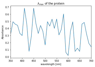
Calculate the extinction coefficient (\(\epsilon\)) of the standards.
The Beer-Lambert Law states that Absorbance is proportional to the concentration of the absorbing molecules, the length of light-path through the medium and the molar extinction coefficient:
\[Abs = \epsilon \cdot c \cdot l\]where:
- \(Abs\) – absorbance
- \(\epsilon\) – light extinction coefficient at max absorption wavelength \(\lambda_{max}\)
- \(c\) – substance concentration
- \(l\) – length of light-path
therefore \(\epsilon\) is equal to:
\[\epsilon = \frac{Abs_{410}}{c \cdot l}\]# Abs_410 = 0.683876
epsilon = 0.683876/(c*1)where c is concentration of the standard.
Determine the concentration of proteins in solution
Knowing epsilon just simply solve standard Beer-Lamber equation for \(c\). Another approach is to construct calibration curve from known samples, determine function, which fits data best and use it to calculate x (concentration) with known y (absorbance).
Calibration curve
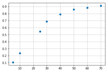
Consider the following example involving a set of six standard points (5, 10, 25, 30, 40, 50, 60, and 70 µg/mL). Absorbance: (0.106, 0.236, 0.544, 0.690, 0.791, 0.861, 0.882, 0.911). I have two columns of x and y values of the calibration curve points.
| Conc. | Abs. | |
|---|---|---|
| 5 | 0.106 | |
| 10 | 0.236 | |
| 25 | 0.544 | |
| 30 | 0.690 | |
| 40 | 0.791 | |
| 50 | 0.861 | |
| 60 | 0.882 | |
| 70 | 0.911 |
It is quite easy to plot this points to visualize data and get some general overview of their shape, like that:
import numpy as np
import matplotlib.pyplot as plt

# Calibration curve data
concentration = np.array([5, 10, 25, 30, 40, 50, 60, 70])
absorbance = np.array([0.106, 0.236, 0.544, 0.690, 0.791, 0.861, 0.882, 0.911])

plt.plot(concentration, absorbance, 'o')
plt.grid(alpha=0.8)
Not bad, six lines of code and plot is ready.
Linear fit
To fit the data to the line I will use scipy package. Linear fit means I will try to find function with general definition:
where:
- \(A\) - is slope
- \(b\) - is intercept
and specific function will have minimal error value fitted for all points with least square regression.
from scipy import stats

slope, intercept, r_value, p_value, std_err = stats.linregress(concentration, absorbance)
Now I will visualize standard curve points and line fitted to them:
# plot of fitted line
plt.plot(concentration, absorbance, 'o', label='data points')
plt.plot(concentration, intercept + slope*concentration, 'r', label='fitted line')
plt.legend()
plt.grid(alpha=0.8)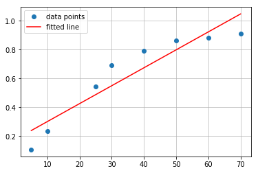
For this set of points linear fitting seems to be suboptimal choice. \(R^2 = 0.8754454029810919\). Lets try other type of function - polynomial.
Polynomial fit
Polynomial fitting may better reflect character of the points. In above data set there is step increase region with more flat part at the top. It would be much better to fit other type of function, which will be able to reflect plateau at the end. Such properties have polynomials or logarithmic functions. Lets try with second degree polynomial known as quadratic function. In this case second degree polynomial is sufficient. Fitting function creates list of coefficients for least-squares fit of the data points to the polynomial function described in general as: \(p(x) = c_0 + c_1 x + … + c_n x_n\):
#polynomial fit
from numpy.polynomial import Polynomial as P

coefs = P.polyfit(concentration, absorbance, 2)
ffit = P.polyval(concentration, coefs)

plt.plot(concentration, absorbance, 'o', label='data points')
plt.plot(concentration, ffit, 'r', label='fitted line')
plt.legend()
plt.grid(alpha=0.8)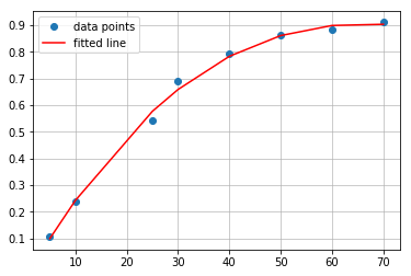
Coefficients are: -0.03969222, 0.03034985, -0.00024301. Therefore polynomial has form:
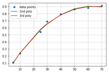
\[y = -0.0396x^2 + 0.0303x - 0.00024\]You can go ahead and write script taking third degree polynomial to fit the data, or run snippet prepared in Jupyter Notebook. As I mentioned before, there is minimal difference between quadratic and cubic fit. Both polynomials comparison should look similar to this:
Concnetration interpolation
Interpolation of the unknown sample is simple as resolving one of the functions in respect to x. In case of linear regression transformation is trivial (rounded to four decimal places):
\[x = \frac{(absorbance - intercept)}{slope} = \frac{(absorbance - 0.176)}{0.0124}\]Lets calculate concentration for 0.5 absorbance:
\[x = \frac{(0.5 - 0.176)}{0.0124} = 26.129\]Althought this is very simple algebra, it can also be replaced by python computations. sympy module allows to perform symbolic math operations like this:
import sympy as smp
smp.init_printing(use_unicode=True)

x, y = smp.symbols('x y')
A, b = smp.symbols('A b', float=True)

y = A*x+b

smp.solveset(y, x)What this lines do? First two import sympy package and set some printing options. Next identify normal python variables x, y, A, b as sympy Symbol() objects. Further expression is set and solved against x. This approach calculates exact x for y equal 0. If I substitute y with some value, I will have to change expression to:
expr = (A*x+b)-y

smp.solveset(expr, x)For second degree polynomial it is little bit more complicated. We can use well known math formula for quadratic equation roots, or ask sympy and numpy to calculate it for us.
To get exact symbolic solution:
x, y = smp.symbols('x y')
a1, a2, a3 = smp.symbols('a1 a2 a3', float=True)

expr = (a1*x**2 + a2*x + a3) - y
smp.solveset(expr, x)
Which results in:
\[\left\{- \frac{a_{2}}{2 a_{1}} - \frac{1}{2 a_{1}} \sqrt{- 4 a_{1} a_{3} + a_{2}^{2}}, - \frac{a_{2}}{2 a_{1}} + \frac{1}{2 a_{1}} \sqrt{- 4 a_{1} a_{3} + a_{2}^{2}}\right\}\]For numeric solution I will solve the equation \(f(x) - y = 0\) using np.roots, where \(f(x)\) is our polynomial:
from numpy.polynomial import Polynomial as P

p = P.fit(concentration, absorbance, 2)
(p - .5).roots()


Out[5]:
array([  21.47501868,  103.41541963])
For absorbance equal 0.5 program returned two values: 21.47501868 and 103.41541963. Quick look at the graph shows that value we are looking for is 21.475.
But why there are two values and how to identify correct one? It is easy If we go back to the fitting and check what kind of function was used to fit data. I used parabola (quadratic), ascending arm of the parabola to be exact. Therefore for each point within x range (5-70) one can expect that quadratic function will have additional solution from descending arm, outside of the x scope. In reality our fitting function looks like this:
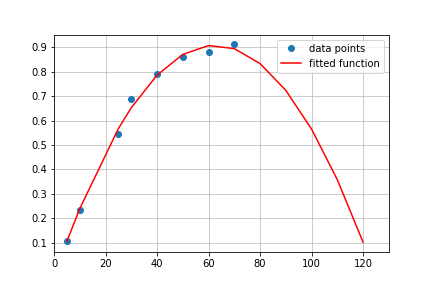
That is why only points fitted within x data range make sense and rest is irrelevant. There is one concern, which is related to the maximum point, which may be placed within x data range and then plateau data may suffer from that, giving wrong results. Possibly for this data set. logarithmic function would be perfect. However from Beer-Lambert law we know, that only linear growth phase from 0.05 to 0.7 absorbance is relevant, thus accuracy of the asymptotic region can be neglected.
Example Jupyter notebook can be downloaded from GitHub.